
Computer Vision 101: Features
What is a ‘feature’ in the context of computer vision? Put concisely it is a visually interesting part of an image.
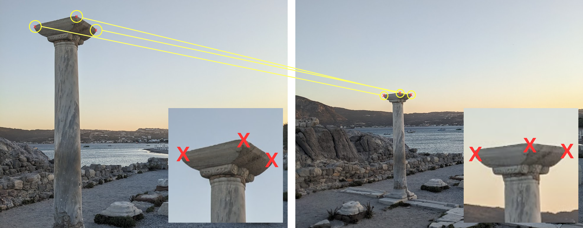
3 features are identified and matched between images
The OpenCV docs use the analogue of piecing a jigsaw puzzle together to highlight the intuition behind features. The idea being in order to connect two pieces together, the puzzle players needs to identify visual features between tiles that might help them relate any two given tiles (often with some additional locking constraint on the piece edges).
This process is abstract, instantaneous and unconscious for the player, but on inspection is actually a sequential and codify-able process:
-
Detect something visually interesting on the tile. For example, the sudden change in colour of a building contrasted by the blue sky horizon above it.
-
Describe the visual feature. This often means looking locally around this visually interesting point. Is there anything that can uniquely describe the visual feature? For example, the angle of the roof relative to the puzzle piece, the colour of the roof, or even the amount of contrast between the roof and sky.
-
Associate or match the current feature’s description (a descriptor) with descriptions generated from visual features on other puzzle tiles. To a puzzle player this would mean looking all the unmatched pieces’ descriptors and then ranking them against the current feature’s description based on similarity. For example, if two pieces show a top of a building behind a blue sky horizon at both at slightly different focal lengths then they are likely to be puzzle piece neighbours.
This process is almost identical for computer vision tasks except the objective is often to find visual descriptors that overlap between images rather than logical continuations of two descriptors. Nonetheless, this analogy acts as a nice construct to view a typical visual feature processing pipeline:
- Feature Detection (identify a feature)
- Feature Description (create a descriptor that describes the local area around the feature)
- Feature Association (go through all descriptors pairwise and match pairs based on description similarity)
Why do all this? Well similar to how you can build a puzzle based on feature associations between puzzle pieces, you can build an understanding of the world based on feature associations between images. For example, analysing how one feature has moved from one frame to another allows you to the determine the relative or absolute position of an object in the real world and even infer its future position.
Feature Detection
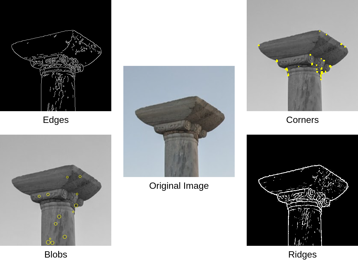
Edges, Corners, Blobs and Ridges are 4 common ‘interest points’ feature detectors look for
What to look for when creating a feature? Common visual features include:
- Edges, formally these are areas of an image where noticeable discontinuities between pixels exist. The ’edge’ being the curve drawn through the border of these discontinuities. Various mathematical methods exist to identify borders of discontinuities including Sobel and Canny edge detectors. The Sobel detector is one of the simplest edge detection methods, where a pair of Sobel kernels are convolved in both X and Y directions – the Sobel kernel effectively takes the difference in pixel values on either side of the convolved patch of the image to provide an ’edge score’ in the X and Y directions. The Canny detector builds on the output of a Sobel kernel by combining Non-Maximum Suppression and Hysteresis Thresholding.
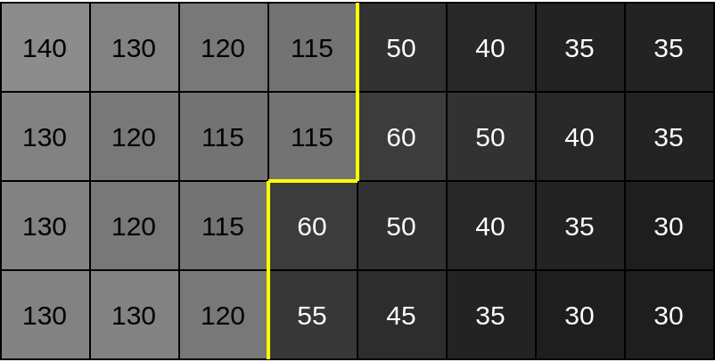
Discontinuity in value between greyscale pixels create an identifiable yellow ’edge'
- Corners are typically found at the intersection of two well-defined edges (in 2D space). The Moravec detector is the simplest corner detection approach, where each part of an image is compared with neighbouring image patches for similarity – if a corner is present it will look quite different to neighbouring image patches, whereas an edge will have a high similarity as it is just a continuation of neighbouring image patches. The Harris detector further builds on the Moravec detector by using a Gaussian window, omni-directionality via a Taylor series expansions (vs. up, down, left, right of Moravec) and eigenvalue analysis for detecting edge intensity.
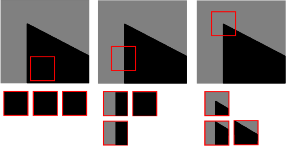
Two well-defined edges meet to form a corner. Measuring the similarity of an image patch vs. its neighbouring image patches can discriminate a corner from and edge. (Vincent Mazet)
- Blobs despite their ambiguous name are just a contiguous group of pixels which share a common property such as colour/intensity value (in case of greyscale). One of the most frequently used approaches builds on differential edge detection methods, specifically using the Scale-Normalised Laplacian of Gaussian. By combining the noise smoothening of a Gaussian and the 2nd derivative of an image (the change of intensity change), you can obtain a 2D-map of blob edge response. When this map is normalised with by the Gaussian’s σ value, the detection of a maxima/minima indicates the location of a blob an its relative scale to σ. However, since the σ value of Gaussian used is correlated to the size/scale of blob, larger σ values (more blur) are needed to detect large blobs and vice versa for smaller blobs (less blur). To counter this several σ values can be tested where new responses indicate new blobs and at different sizes, this is often referred to as a Multi-Scale Laplacian of Gaussian.
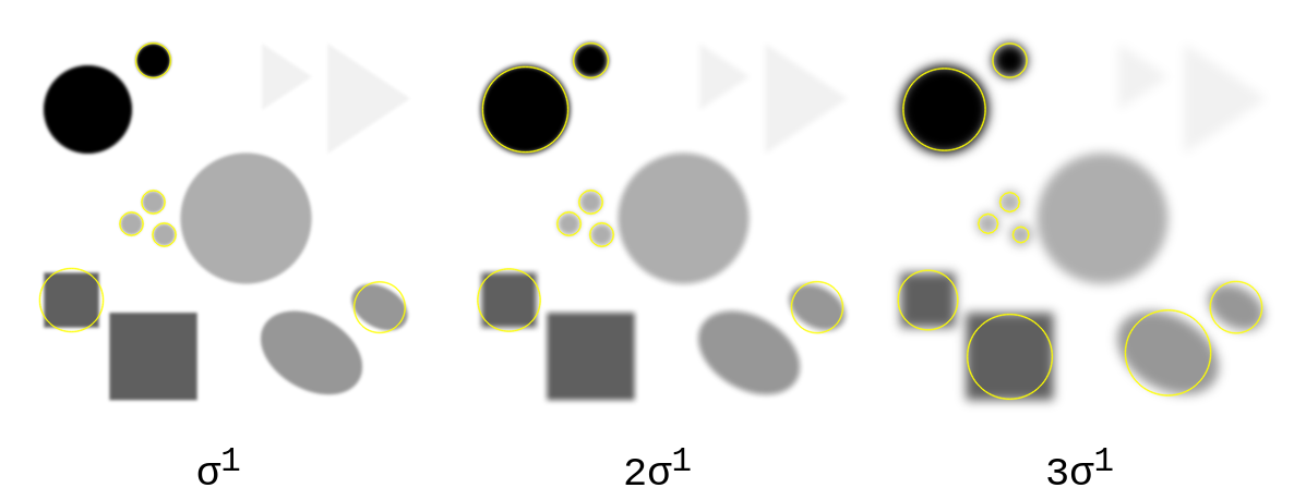
As σ gets larger, blobs of larger size are detected – Scale-space representation
- Ridges, unlike edges, are found when the intensity of an image peaks. For example, the ridge on the top of a mountain range when seen top-down from satellite image. In fact common ridge detection setting include detecting roads in aerial images, blood vessels in retinal images, patterns in fingerprints, crack detection amongst other applications. Most ridge detectors use some form of Hessian matrix analysis where the 2nd derivative of an image (the change of intensity) acts as the inputs to the Hessian. As the Hessian describes information about the curves of image intensity, the eigenvalues and eigenvectors can be analysed to detect a rapid change of gradient – indicative of passing over a ridge.
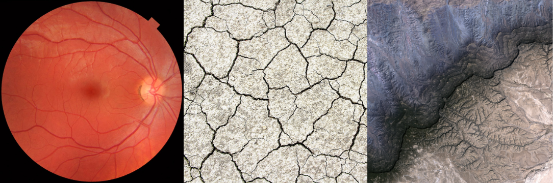
Typical examples of images where ridge detection is favoured
Various other features exist such as Texture features, Optical flow features etc. but on inspection often build on the primitives of Edges, Corners, Blobs and Ridges.